Creating single-level simulations
Starting from scratch
All simulations should be placed in the exec folder. To begin setting up a new simulation, use the spawn shell script. For example, suppose you want to create a 2D internal wave simulation on a computer with 16 available processors.
$ cd exec
$ ./spawn MyFirstProject
This will create a somar/exec/MyFirstProject folder that is populated with several files that are ready to compile and run. To compile the default code with the GCC compiler suite, do the following.
$ cd MyFirstProject
$ ./buildall -j32 --D=2 --Serial
Although our computer has 16 available processors, we may have 2 threads per core, so we request twice as many simultaneous jobs when compiling with the -j32 option. If you wish to use the Intel or Clang compiler suites, add the --IntelCompiler or --Clang flags to the buildall command.
If all goes well, an executable will be created named Somar_2D.Serial.gcc.ex. By default, this simulation will not do much because the initial state will be set to zero. Nevertheless, we should run it just to be sure everything is working.
$ ./Somar_2D.Serial.gcc.ex inputs.template.machine > std.out
Within std.out, we should see some convergence metrics, energy calculations, and so on. We will sort much of this out later. For now, you should check that the file concludes as expected.
########################### AnisotropicAMR::conclude ###########################
checkpoint file name = check_points/chkpt_000001.2d.hdf5
number of points updated at level 0 = 4096
total number of points updated = 4096
If so, SOMAR is properly set up on your system for serial runs.
If MPI is available on your system, the compilation process is similar. In fact, there are only 2 changes that need be made. First, MPI is the default mode, so remove the --Serial flag from the build line. Second, the executable will have a slightly different name.
$ ./buildall -j32 --D=2
$ mpirun -np 16 ./Somar_2D.MPI.gcc.ex inputs.template.machine
You can still pipe the standard output to a file, but there is less need to do so in MPI mode as most of the information will be written to files for us. SOMAR now generates several pout.* files, one for each MPI rank. This is where Poisson solver convergence info and other diagnostic information will be written. The terminal will only display very basic info to let you know how far along the simulation has progressed.
Setting the EoS and initial conditions
The main C++ class used by SOMAR is the AMRNSLevel class. A class is just a collection of data and functions, and AMRNSLevel contains all of SOMAR’s state data and functions that help compute the RHS of the Navier-Stokes equations. A peek inside somar/src/Grade5_SOMAR/AMRNSLevel.H will reveal a wealth of functionality. Do not get overwhelmed! Most simulations override the same handful of functions. As you learn to use SOMAR, you’ll find that you typically just need to set initial and boundary conditions, set a permanent background stratification, adjust the equation of state, and perhaps, add some scalars or a forcing function. Over time, you’ll end up becoming very familiar with a common set of functions and learn to ignore the rest. For now, we will direct our attention to just two commonly used functions, equationOfState and setICs.
Customizing the EoS
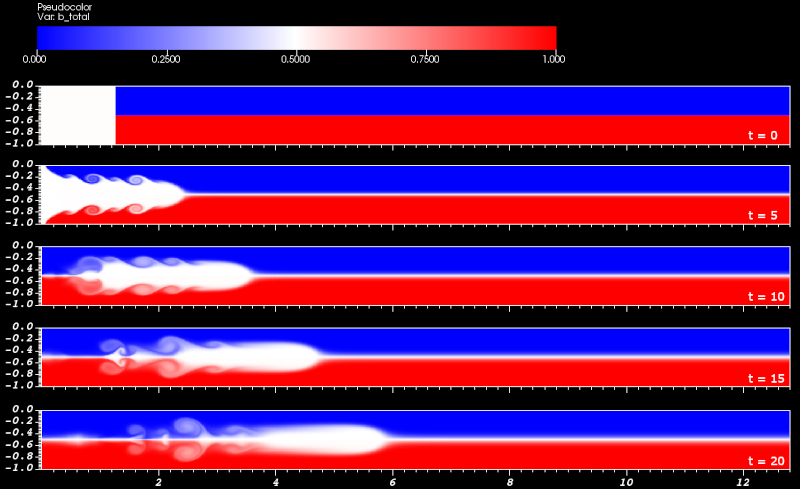
Let’s set up a simple two-layer internal wave simulation with lighter fluid on top, heavier fluid on the bottom, and a mixed region on the left. The mixed layer will push its way across the domain between the lighter and heavier fluid.
SOMAR does not deal with density directly. Instead, we need to specify the initial temperature and salinity so that SOMAR can compute the reduced gravity via an equation of state, \(b = g(\rho-\rho_0)/\rho_0 = \Gamma(T,S)\). By default, SOMAR uses the linear equation of state
Warning
Technically, buoyancy is defined as the negative of our reduced gravity. Nevertheless, we will call \(b = g(\rho-\rho_0)/\rho_0 = \Gamma(T,S)\) the buoyancy field. Keep this in mind when greating custom equations of state!
For our example, we want to abandon this default EoS and let the temperature be a proxy for the buoyancy by setting \(\Gamma(T,S) = T\). To do this, we must override the equationOfState function by placing the following code in your UserPhysics class within the UserPhysics.H file.
/// Our custom EoS. This simply sets b = T.
virtual void
equationOfState(FArrayBox&       a_bFAB,
                const FArrayBox& a_TFAB,
                const FArrayBox& a_SFAB,
                const FArrayBox& a_zFAB) const override
{
    a_bFAB.copy(a_TFAB);
}
Note
In C++, it is considered good practice to split the declaration and implementation of a function. There are a few exceptions to this rule. One exception is when the function implementation is very small (one or two lines long). Defining a small function within its declaration might allow the compiler to inline the function and eliminate the call, bringing pros and cons that are beyond the scope of this tutorial.
Setting the ICs
Next, we turn to the initial conditions. Because all simulations need initial conditions, the setICs function was created for you by the spawn utility. Open UserPhysics.cpp and update the setICs as follows.
void
UserPhysics::setICs(State& a_state)
{
    // NOTE:
    // In this simple example, remember that there is no temperature.
    // T is just a proxy for b. That is why we fill T with b values!
    // In other words, we set a_state.T with b_total!

    // As is, our code will only work in 2D.
    CH_verify(SpaceDim == 2);

    // Gather geometric info.
    const DisjointBoxLayout& grids = m_levGeoPtr->getBoxes();
    const Real               L     = m_levGeoPtr->getDomainLength(0);
    const Real               x0    = 0.1 * L;
    const Real               z0    = -0.5;

    // Loop over each grid in the layout...
    for (DataIterator dit(grids); dit.ok(); ++dit) {
        // Create references to this grid and this grid's data holder.
        const Box valid = grids[dit];
        FArrayBox& TFAB = a_state.T[dit];

        // Loop over each cell in the grid...
        for (BoxIterator bit(valid); bit.ok(); ++bit) {
            const IntVect& iv = bit();
            const Real     x  = m_levGeoPtr->getCellX(0, iv);
            const Real     z  = m_levGeoPtr->getCellX(1, iv);

            // The vertical structure.
            if (z > z0) {
                TFAB(iv) = 0.0;
            } else {
                TFAB(iv) = 1.0;
            }

            // The mixed region.
            if (x < x0) {
                TFAB(iv) = 0.5;
            }
        }
    }
}
This should compile and run without issue, but we still have a few more details we need to address. Our interface location of \(z_0 = -0.5\) is meaningless until we set up the computational domain. This can be done in the input file.
The input file
The spawn utility automatically populates your input file template with an organized list of tweakable parameters. Most of them are commented out using the # character. When a parameter is commented out, we allow SOMAR to use a default value. For example, your input file contains this line.
# time.maxDt = 0.5 # [1.0e8]
The # character at the start of the line ensures amr.maxDt is not read from this input file and the default value of 1.0e8 (shown at the right) is used. If we uncomment this line, we can manually set a more reasonable value. All parameters whose line ends with # MUST SPECIFY have no default value. Be sure to set these values.
The input file is divided into groups, or prefixes. Each prefix controls a different aspect of your simulation.
Prefix |
What it controls |
|---|---|
base |
Base level geometry, resolution, and decomposition details. |
time |
Time stepping controls – dt limits, max number of steps, restart details, etc. |
output |
Controls plots, checkpoints, and other diagnostic info. |
amr |
Adaptive refinement controls. |
rhs |
Model parameters – viscosity/diffusivities, BCs, forcing toggles, LES controls, etc. |
proj |
Projector parameters – conergence tolerance, multigrid and relaxation details, etc. |
strat |
Background stratification parameters. |
ib |
Immersed boundary parameters. |
Knowing this, let’s set up our 2D internal wave simulation using a channel with dimensions \((12.8, 1)\), with the top and bottom located at \(z = 0\) and \(z = -1\), respectively. To resolve the flow, we will discretize the domain into \((1024, 128)\) cells and increase the viscosity/diffusion to \(10^{-4}\). Once the flow begins, SOMAR will compute that the maximum stable timestep is approximately 0.02, limited by the advection scheme. To be on the safe side, we will scale this by 0.9.
Note
I am not attempting to provide scales that are physically relevant in any way, so I will not include units unless there is an elucidating reason to do so.
In your input file, locate and set the following parameters.
#------------------- Base level geometry and decomposition --------------------#
base.L        = 12.8 1.0           # MUST SPECIFY
base.nx       = 1024 128           # MUST SPECIFY
base.nxOffset = 0 -128             # [0 0 0]

#---------------------------- Timestepping details ----------------------------#
time.stopTime = 100.0
time.maxSteps = 2000
time.maxDt    = 0.1                # [1.0e8]
time.dtMult   = 0.90               # [0.80]

#------------------------------ Model parameters ------------------------------#
rhs.nu        = 0.0001             # [0.]
rhs.TKappa    = 0.0001             # [0.]
Using base.L and base.nx, we can calulate the cell sizes along with the physical coordinates of the nodes and cell-centers.
Warning
These formula are only true in a simple, unstretched, Cartesian coordinate system. We will revisit these formulas when we introduce grid stretching.
In 2D, each cell has 4 vertex nodes. The node at the lower left of each cell shares its index with the cell-center. Notice that \(z=0\) is at the \(j=0\) nodes, which is why we vertically shift the domain using base.nxOffset. This can be a point of confusion, so let’s elaborate.
By setting base.nxOffset = 0 -128, we shift the cell indices from \((i,j)_{\rm{cells}} = (0,0)..(1023, 127)\) to \((0,-128)..(1023, -1)\). Similarly, the nodal indices shift from \((i,j)_{\rm{nodes}} = (0,0)..(1024, 128)\) to \((0,-128)..(1024, 0)\). So, by vertically shifting the domain, the bottom nodes are at \(z_{-128} = -128 \Delta z = -128 \cdot (1/128) = -1.0\) and the top nodes are at \(z_{0} = 0 \cdot \Delta z = 0\).
One last point about resolution and load balancing. Our domain is discretized into 1024-by-128 cells. This divides nicely into \(2^p\)-by-\(2^p\) blocks. This simulation will have a balanced load if we use 1, 2, 4, 8, 16, or even 32 MPI ranks. If you choose a number of MPI ranks that does not allow a balanced load, a warning will be emitted at the start of the simulation along with a suggestion. Choosing appropriate settings to obtain fast and balanced simulations is tricky. Especially when multigrid is used to solve the pressure Poisson problem. We will save this conversation for later. For now, we will rely on SOMAR to do the load balancing.
Visualizing the output
By default, the output will be written to the hdf5_output folder within your project folder. If you’d like to change the default location or change the amount of data generated, change the following parameters.
output.plotInterval    = 1                   # [-1]       MUST SPECIFY THIS
output.plotPeriod      = -1.0                # [-1.0]     OR THIS!
output.plotPrefix      = hdf5_output/plot_   # [plot_]
The output.plotPrefix setting controls where to save the data relative to the simulation’s working directory. In this example, the files will be named plot_000000.2d.hdf5, plot_000001.2d.hdf5, plot_000002.2d.hdf5, and so on. The other two parameters control when to save data.
For example, setting output.plotInterval = 1 will emit a data file at each timestep. Setting this to 5 will emit a data file every 5 timesteps. Setting output.plotPeriod = 0.25 will emit a data file at \(t = 0.0s, 0.25s, 0.50s, 0.75s, \dots\) Typically, you would set one or the other, but not both.
The data is written to HDF5 files in a format that is native to the Chombo library that forms the backbone of SOMAR. These files can be opened and visualized using VisIt.
Open visit, click File → Open file, and a dialog box will appear. Navigate to your data’s directory and ensure “Smart grouping” is checked. This will allow you to open the entire time series of data. Click OK and you’ll notice the “Active Source” is set to the plot_*.hdf5 database. Next, we need to choose how to view our data. Let’s take a look at the reduced gravity (called buoyancy in SOMAR). Click the Add → Pseudocolor → b_total, then click “Draw”. An image of the initial conditions should appear in the visualization window. To move to another timestep, adjust the “Time” slider. For more information about how to visualize data in VisIt, feel free to play around or go to the VisIt website.
Importing data from Matlab
Next, let’s convert our simple internal wave simulation to model an internal solitary wave of depression traveling to the right in a continuously stratified fluid. The theory behind these waves are by no means trivial and the reader is encouraged to read [StastnaLamb2002] for details. For the purposes of this tutorial, the initial conditions are provided in a text file that can be read by SOMAR. You can download the file here.
Reading initial conditions from a data file is such a common task that SOMAR provides the IO::readASCII function to help. This function can read space/new-line separated data from a text file and store it in either a std::vector or a LevelData<FArrayBox>. For example, here is how to read the first 20 real numbers from MyDataFile.txt. The first 12 will be placed into v1 and the remaining 8 will be placed into v2.
#include <IO.H> // At top of file.

// ...

// Open the input file
const std::string filename("MyDataFile.txt");
std::ifstream inFile(filename);
if (!inFile.is_open()) {
    MAYDAYERROR("Could not open file " << filename << ".");
}

// Read the first 12 real numbers.
std::vector<Real> v1(12);
IO::readASCII(v1, inFile);

// Read the next 8 real numbers.
std::vector<Real> v2(8);
IO::readASCII(v2, inFile);

// We are done.
inFile.close();
To read a 2D or 3D array of data, the code is similar. This snippet shows how to read cell-centered velocity components from the file.
// Read an entire domain of CC velocity data.
LevelData<FArrayBox> ccVel(grids, SpaceDim);
for (int velComp = 0; velComp < SpaceDim; ++velComp) {
    IO::readASCII(ccVel, velComp, inFile);
}
Warning
Behind the scenes, IO::readASCII reads the data on a single processor, then distributes the data onto your processor layout. So, remember that this is a serial operation that should be called sparingly!
In SOMAR, velocity components are face-centered and all other scalars are cell-centered (SOMAR uses Arakawa-C grids. See: [ArakawaLamb1977]). This means we need to recenter the velocity components. Typically, we do this by filling a ghost layer, then using standard second-order averages.
// At top of file.
#include <BCTools.H>
#include <Convert.H>
#include <IO.H>

// ...

// Read CC vel.
LevelData<FArrayBox> ccVel(grids, SpaceDim, IntVect::Unit);
for (int velComp = 0; velComp < SpaceDim; ++velComp) {
    IO::readASCII(ccVel, velComp, inFile);
}

// Extrapolate and exchange all ghosts.
const int extrapOrder = 2; // Quadratic extrapolation.
BCTools::extrapAllGhosts(ccVel, extrapOrder);
ccVel.exchange();

// Send to FC.
const bool doValidOnly = true;
Convert::CellsToFaces(a_state.vel, ccVel, doValidOnly);
This is a fine way to recenter the velocity, but it requires the simulation’s resolution to be the same as the input data’s resolution. Another option is to use the LinearInterp function, which can both recenter data and change the resolution. The one caveat is that the file’s data cannot be decomposed over many MPI ranks – all data must be available on all ranks during interpolation, creating a resource bottleneck for very large datasets. Later versions of SOMAR will address this issue if it proves to be a problem.
Okay, it’s time to put it all together. In your input file, be sure to have the following parameters set.
#------------------- Base level geometry and decomposition --------------------#
base.L        = 128.0 1.0          # MUST SPECIFY
base.nx       = 1024 128           # MUST SPECIFY
base.nxOffset = 0 -128             # [0 0 0]

#---------------------------- Timestepping details ----------------------------#
time.stopTime = 100.0
time.maxSteps = 2000
time.maxDt    = 0.1                # [1.0e8]
time.dtMult   = 0.90               # [0.80]

#------------------------------ Model parameters ------------------------------#
rhs.nu        = 0.000001           # [0.]
rhs.TKappa    = 0.000001           # [0.]
We reduced the viscosity/diffusion values to \(10^{-6}\) because solitary waves are not driven by diffusive effects. Elevated values will only serve to diffuse the vertical stratification, which we’d like to prevent! The UserPhysics::setICs function should be updated as well.
// At top of file.
#include "UserPhysics.H"
#include "Convert.H"
#include "IO.H"
#include "BilinearInterp.H"

// ...

void
UserPhysics::setICs(State& a_state)
{
    // In this simple example, remember that there is no temperature.
    // T is just a proxy for b. That is why we fill T with b values!
    // In other words, we set a_state.T with b_total!

    CH_verify(SpaceDim == 2); // The text file contains 2D data.


    // Gather data from file -----------------------------------------------
    // The input file's info.
    const std::string filename("DJLIC_1024x128_1.txt");
    const int srcNx = 1024;
    const int srcNy = 128;

    // The lower-left indices of srcDomBox are irrelevant. IO::readASCII
    //  only care's about this Box's size. So feel free to use 1-based
    //  indices here.
    const Box srcDomBox(IntVect(D_DECL(1, 1, 1)),
                        IntVect(D_DECL(srcNx, srcNy, 1)));

    // Open the input file.
    std::ifstream inFile(filename);
    if (!inFile.is_open()) {
        MAYDAYERROR("Could not open file " << filename << ".");
    }

    // x
    std::vector<Real> srcx(srcNx);
    IO::readASCII(srcx, inFile);

    // y
    std::vector<Real> srcy(srcNy);
    IO::readASCII(srcy, inFile);

    // u, w.
    // FArrayBoxes are NOT decomposed like LevelData<FArrayBox>es!
    // This reads the entire domain on all MPI ranks, as discussed.
    FArrayBox srcVelFAB(srcDomBox, SpaceDim);
    for (int velComp = 0; velComp < SpaceDim; ++velComp) {
        IO::readASCII(srcVelFAB, velComp, srcDomBox, inFile);
    }

    // T
    FArrayBox srcTFAB(srcDomBox, 1);
    IO::readASCII(srcTFAB, 0, srcDomBox, inFile);

    // We are done with the file.
    inFile.close();


    // Interpolate data to our grids ---------------------------------------
    const DisjointBoxLayout& grids  = m_levGeoPtr->getBoxes();
    for (DataIterator dit(grids); dit.ok(); ++dit) {
        // vel
        for (int velComp = 0; velComp < SpaceDim; ++velComp) {
            const Box fcValid = grids[dit].surroundingNodes(velComp);
            const auto statex = m_levGeoPtr->getX(0, fcValid);
            const auto statey = m_levGeoPtr->getX(1, fcValid);

            // This aliases a single velocity component.
            const FArrayBox srcVelCompFAB(Interval(velComp, velComp),
                                          srcVelFAB);

            LinearInterp(a_state.vel[dit][velComp],  // dest FAB
                        { statex, statey },          // dest coordinates
                        fcValid,                     // dest Box
                        srcVelCompFAB,               // src FAB
                        { srcx, srcy },              // src coordinates
                        srcDomBox);                  // src Box
        }

        // T
        {
            const Box ccValid = grids[dit];
            const auto statex = m_levGeoPtr->getX(0, ccValid);
            const auto statey = m_levGeoPtr->getX(1, ccValid);

            LinearInterp(a_state.T[dit],     // dest FAB
                        { statex, statey },  // dest coordinates
                        ccValid,             // dest Box
                        srcTFAB,             // src FAB
                        { srcx, srcy },      // src coordinates
                        srcDomBox);          // src Box
        }
    }  // dit
}
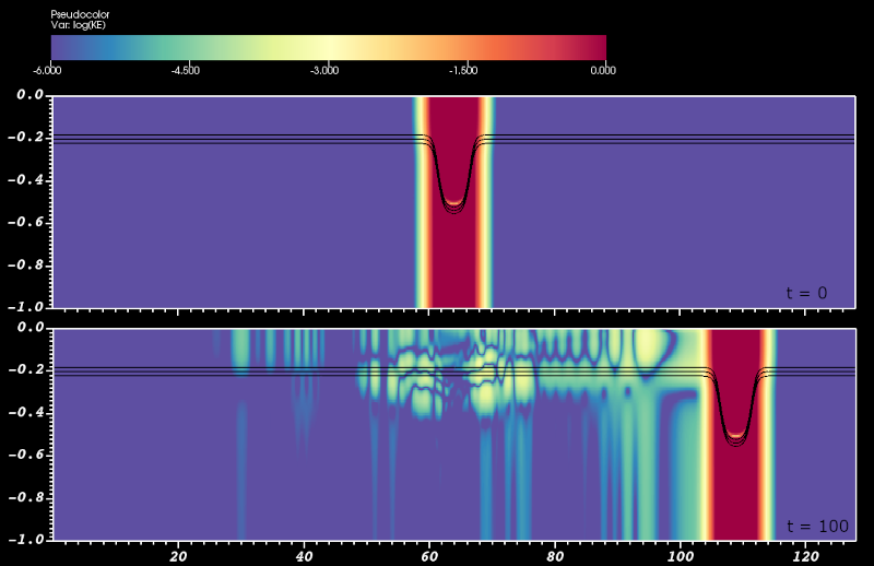
This code should compile and run without error. The images below show the results. The pseudocolor plots are the \(log_{10}(KE)\) clipped to a range of \([-6, 0]\). The three contours are the total buoyancy at values of -0.4, -0.5, and -0.6.
Hopefully, the IO::readASCII function makes some sense. It was designed to work nicely with data prepared by Matlab and GNU Octave. For example, if I have a vector, x, and 2D array, T, in Matlab that I want to write to file for SOMAR, I can do so as follows.
fid = fopen('MyDataFile.txt', 'W');

fprintf(fid, '%f ', x(:));

for k=1:NZ
    fprintf(fid, '%f ', T'(:,k));
    fprintf(fid, '\n');
end

fclose(fid);
Since each call to Matlab’s fprintf function flushes the buffer, we improve performance by filling the buffer with an entire slice of data, T'(:,k), in each fprintf call.
Adding a background stratification
Sometimes, we can view the temperature and salinity as a small perturbation atop a static vertical background profile, \(q(x,y,z,t) = \bar{q}(z) + q'(x,y,z,t)\). (We will use the generic variable \(q\) when referencing some arbitrary subset of the cell-centered scalar fields.) This often makes sense when dealing with stratified flows – the unperturbed stratification is often maintained through unmodeled phenomena and should not be diffused. If SOMAR knows the functions \(\bar{T}(z)\) and \(\bar{S}(z)\), it will diffuse the perturbation rather than the total temperature and salinity as shown here.
Although we did not explicitly specify the vertical profile of the temperature field, a typical tanh profile was provided in the input file. Remembering that our “temperature” variable is actually the buoyancy, the unperturbed stratification is given by
where \(z_0 = -0.2\) is the location of the temperature/density interface and \(\sigma = 0.1\) is the interfacial thickness. SOMAR can automatically generate a linear or tanh background profile via the input file.
# strat.type     = 1              # [0] 0 = NONE, 1 = LINEAR, 2 = TANH
# strat.T0       =                # The value at z = 0.
# strat.dTdz     =                # The upward derivative (typically negative)
# strat.S0       =                # ditto
# strat.dSdz     =                # ditto

strat.type     = 2                # [0] 0 = NONE, 1 = LINEAR, 2 = TANH
strat.T0       = 0.5              # Value at the specified z0 location.
strat.dT       = 0.5              # dT = T_bottom - T_top.
strat.S0       = 0.0              # ditto
strat.dS       = 0.0              # ditto
strat.z0       = -0.20            # The location of the cline's center.
strat.sigma    = 0.1              # The cline's thickness.
This shows the relevant parameters that need to be set for both linear and tanh profiles. Note that strat.T0 and strat.S0 have slightly different meanings in each case. Here, we use a tanh profile with the parameters set to mimic our DJL solitary wave’s ambient stratification. Running SOMAR with these parameters will produce almost identical results with a few notable exceptions.
An extra file,
plot_stratData_lev0.hdf5will appear in your output folder. It contains a \((1,1,N_z)\) line of data describing the scalars’ vertical profiles.The diagnostic info written to the terminal will compute the total energy using the available potential energy (APE) rather than the full gravitational potential energy. Details about APE can be found in [ScottiWhite2006].
Unwanted deterioration of the vertical profile will be avoided when using an elevated diffusivity or SOMAR’s LES features.
The gravitational force will be computed using \(b' = \Gamma(T', S')\) rather than the full buoyancy. This removes the hydrostatic component from the pressure field, simplifying the job of the projector.
If you need use a custom background stratification (not linear or tanh), you can do so by overriding the AMRNSLevel::setStratification function. For example, suppose you want a two-layer structure without a smooth transition.
void
UserPhysics::setStratification(std::vector<Real>& a_vTbar,
                               std::vector<Real>& a_vSbar,
                               std::vector<Real>& a_vz,
                               const Real         a_zmin,
                               const Real         a_zmax) const
{
    // Set T(z) = 1.0 on [a_zmin, -0.5) and
    //            0.0 on (-0.5, a_zmax).
    // We will need 4 control points.
    // Intermediate values will be set via linear or cubic splines.

    const Real z0    = -0.2;
    const Real sigma = 1.0e-4;  // The interface is less than the cell size,
                                // simulating a step function.

    a_vz.resize(4);
    a_vTbar.resize(4);
    a_vSbar.resize(4);

    a_vz[0]    = a_zmin;           // The min z used by SOMAR. Considers ghosts!
    a_vTbar[0] = 1.0;              // Want T_bottom = 1.
    a_vSbar[0] = 0.0;              // Not using salinity.

    a_vz[1]    = z0 - 0.5 * sigma; // Just below the middle of the domain.
    a_vTbar[1] = 1.0;              // Still in bottom layer.
    a_vSbar[1] = 0.0;              // Not using salinity.

    a_vz[2]    = z0 + 0.5 * sigma; // Just above the middle of the domain.
    a_vTbar[2] = 0.0;              // In top layer.
    a_vSbar[2] = 0.0;              // Not using salinity.

    a_vz[3]    = a_zmax;           // The max z used by SOMAR. Considers ghosts!
    a_vTbar[3] = 0.0;              // In top layer.
    a_vSbar[3] = 0.0;              // Not using salinity.
}
You can create as many control points as you like. By default, intermediate values will be linearly interpolated. If you’d like to use cubic splines, add the input parameter strat.interpOrder = 3. Cubic interpolation works nicely when there are no large jumps and many control points.
By modifying this function, you can create any background stratification you need. You can even prepare your data in Matlab and use IO::readASCII to import it. This is very useful when dealing with a realistic stratification from a lab tank or the ocean.
In the remaining sections, we will return to the pre-packaged tanh stratification.
Note
SOMAR is based on the Chombo library, which defines the Vector class. SOMAR also uses the C++17 standard library, which provides the std::vector class. To prevent confusion, we’ve ensured that there is no distinction between the two. One is just an alias of the other.
Stretching the grids
So far, we’ve been working in a simple, uniform Cartesian coordinate system generated by (1). SOMAR allows you to displace each of the nodes in the domain to create a non-uniform, or stretched, coordinate system. Unfortunately, the coordinate system must be known very early in the SOMAR’s initialization, so creating a custom geometry involves a bit more work than simply overriding a function. To understand this, let’s take a moment to talk about a core-concept in C++, inheritance.
An aside about inheritance in C++
Open up src/Grade5_SOMAR/AMRNSLevel.H. Do not edit it, just have a look around. There’s some boilerplate stuff like licensing info and include directives, but at about 100 lines in, a class called AMRNSLevel is defined. Within this class are a myriad of functions that initialize the grids, calculate the timestep, estimate the pressure, set BCs, and so on. Every tool we need to solve the Navier-Stokes equations is declared and defined within this class. You’ll even notice some familiar functions like AMRNSLevel::equationOfState.
So, SOMAR expects to be handed an AMRNSLevel object so that it can call all of these functions to solve the Navier-Stokes equations. AMRNSLevel defines much of SOMAR’s default functionality. Now, here’s the sneaky part. C++ allows us to create a child class that inherits all of the default functionality we need and override the rest. This is where our UserPhysics class steps in. At its core, it just inherits all of AMRNSLevel’s’ functions. However, we’ve been customizing some of this functionality when we created our UserPhysics::equationOfState, UserPhysics::setICs and setStratification functions. Whenever SOMAR needs to evaluate the equation of state, it calls our customized version rather than the default version. This is one of the things that makes C++ so powerful. If you want to change the bahavior of any piece of SOMAR, you’ll often find yourself just overriding one of AMRNSLevel’s functions in your UserPhysics class.
But wait, how does SOMAR know about our custom physics class? Well, when we used the spawn utility to create a bare-bones project, it created a UserMain.cpp file containing two functions: UserMain::oneTimeSetup and UserMain::createPhysics. Notice that the latter creates a UserPhysics object and returns it back to SOMAR as the AMRNSLevel object it expects! As long as our custom physics class is a child of AMRNSLevel, SOMAR can’t tell the difference.
Creating a very basic geometry class
So, what does this have to do with grid stretching?! Well, take a look at the UserMain::oneTimeSetup function. Its job is to perform whatever initialization is needed before the AMRNSLevel object is created, like defining a coordinate system. GeoSourceInterface is the parent class that declares all of the functions that SOMAR will expect of a coordinate system. Much like AMRNSLevel, it contains a few functions we will need to override and many we do not. Ultimately, there are three functions that must be overridden. This is indicated by the = 0 at the end of their declaration. GeoSourceInterface provides no default functionality for these functions.
class GeoSourceInterface
{
public:
    /// Default destructor
    virtual ~GeoSourceInterface ();

    // -------------------------------------------------------------------------
    /// \name These must be overridden
    /// \{

    /// 1. Must return the name of the coordinate mapping
    virtual const char* getCoorMapName () const = 0;

    /// 2. Must return whether or not this metric is uniform
    virtual bool isUniform () const = 0;

    /// 3. Interplates the function x^mu(xi^mu).
    virtual void interp(std::vector<Real>&       a_x,
                        const std::vector<Real>& a_xi,
                        const int                a_mu) const = 0;
    /// \}

    // -------------------------------------------------------------------------
    /// \name These can be overridden if the analytic functions are known.
    /// \{

    /// Computes the physical coordinates of the cells or nodes of a box.
    virtual void fill_physCoor (std::vector<Real>& a_x,
                                const int          a_mu,
                                const Real         a_dXi,
                                const Box&         a_box) const;

    // ...
Now, let’s create our own custom geometry. Create two files in your project’s directory, MyStretchedMap.H and MyStretchedMap.cpp – a header file and an implementation file. In the header file, add the following code.
#pragma once
#include "GeoSourceInterface.H"

class MyStretchedMap : public GeoSourceInterface
{
public:
    /// Constructor
    MyStretchedMap();

    /// Destructor
    virtual ~MyStretchedMap();

    /// 1. Must return the name of the coordinate mapping
    virtual const char*
    getCoorMapName() const override;

    /// 2. Must return whether or not this metric is uniform
    virtual bool
    isUniform() const override;

    /// 3. Interplates the function x^mu(xi^mu).
    virtual void
    interp(std::vector<Real>&       a_x,
           const std::vector<Real>& a_xi,
           const int                a_mu) const override;
};
Notice that this inherits from GeoSourceInterface, which requires us to provide an implementation for the last three functions. The first two functions are called the constructor and destructor. They tell C++ how to properly create and destroy our MyStretchedMap objects. Do not rely on inheritance here – you should always create a non-virtual constructor and a virtual destructor.
Note
Constructors and destructors in the face of inheritance is a tricky thing. This document is no substitute for actually learning C++! Luckily, most of SOMAR’s use cases only require a basic understanding of inheritance. Most of the time, you’ll just be inheriting from AMRNSLevel and occasionally, you’ll need to create a custom geometry class.
Now, let’s move on the the implementation. In the corresponding .cpp file, add the following.
#include "MyStretchedMap.H"

// -----------------------------------------------------------------------------
MyStretchedMap::MyStretchedMap()
{
    // Do nothing for now.
}


// -----------------------------------------------------------------------------
MyStretchedMap::~MyStretchedMap()
{
    // Do nothing for now.
}


// -----------------------------------------------------------------------------
const char*
MyStretchedMap::getCoorMapName() const
{
    return "MyStretchedMap";
}


// -----------------------------------------------------------------------------
bool
MyStretchedMap::isUniform() const
{
    return false;
}


// -----------------------------------------------------------------------------
void
MyStretchedMap::interp(std::vector<Real>&       a_x,
                       const std::vector<Real>& a_xi,
                       const int                a_mu) const
{
    a_x = a_xi;
}
Most of these functions are quire simple and self-explainatory, but the last function needs to be discussed. SOMAR bounces back and forth between two coordinate systems, logical and physical coordinates. The logical coordinates of each node are always defined by
and the logical coordinates of each cell-center are defined similarly, but with 1/2 added to the index. If these relations look very similar to the unstretched Cartesian coordinates defined by (1), it’s because in unstretched coordinates, the logical and physical coordinates are identical. In a stretched system, the next step is to override the GeoSourceInterface::interp function to do our bidding – to take the unstretched, logical coordinates \((\xi, \eta, \zeta)\), and compute the physical coordinates \((x,y,z)\). In the above code, we set the physical coordinates to the logical coordinates. This leads to no stretching at all, which is good enough for the moment. We’ll return to this function in a moment to define something a bit more interesting. For now, let’s tell SOMAR to use our new code in place of the GeoSourceInterface that it expects.
Open your project’s UserMain.cpp file. Near the top of the file, include our new geometry’s header file. Then, in USerMain::oneTimeSetup, create a new MyStretchedMap object and return it to SOMAR.
GeoSourceInterface*
UserMain::oneTimeSetup ()
{
    ProblemContext* __nowarn_unused ctx = ProblemContext::getNonConstInstance();
    // Alter the default parameters, if needed. Or, stash important info
    // needed by your user-defined physics class.
    // ...

    // Create and return a coordinate system.
    // By default, we create a simple, uniform, Cartesian coordinate system.

    // CartesianMap* geoPtr = new CartesianMap(); // <------ Commented out!!
    MyStretchedMap* geoPtr = new MyStretchedMap();

    return geoPtr;
}
This should compile and run. The results of the simulation should be identical to the results that used the unstretched CartesianMap. If all is running smoothly, we’re ready for the last part. We are ready to supply a stretching function to our MyStretchedMap::interp function.
Customizing our geometry class
As previously mentioned, the MyStretchedMap::interp function defines the mapping between the logical and physical coordinates via two functions (or three functions in 3D),
In our 2D DJL example, we’d like to focus the grids at the pycnocline, at \(y = -0.2\) non-dimensional units. The stretcing function we will use is rather complex, but it does the job. The x-coordinate is not stretched, the z-coordinate is not used (this is a 2D simulation), and the y-coordinate will obey
And here is a possible implementation.
void
MyStretchedMap::interp(std::vector<Real>&       a_x,
                       const std::vector<Real>& a_xi,
                       const int                a_mu) const
{
    // a_mu tells us the coordinate direction. (0 = x, 1 = y)
    if (a_mu == 1) {
        for (size_t idx = 0; idx < a_x.size(); ++idx) {
            const Real eta = a_xi[idx];
            const Real arg = std::pow(eta + 1.0, 3);
            const Real s  = tanh(1.7 * (arg + 0.1));
            const Real s0 = tanh(1.7 * (0.0 + 0.1));
            const Real s1 = tanh(1.7 * (1.0 + 0.1));

            a_x[idx] = 1.0 + 2.0*eta - (s - s0) / (s1 - s0);
        }
    } else {
        // Do not stretch the grids in other directions.
        a_x = a_xi;
    }
}
Note
C++ is very good at optimizing well written code. Unfortunately, some necessities in Fortran are bad habits in C++.
Do not be tempted to declare all variables at the start of a function. Instead, give them the smallest scope possible. See how we created our variables inside the loop? That was no accident!
Use
constliberally. By telling C++ that a variable should not change, you are allowing the compiler to make more aggressive optimizations. It may even optimize the variables away altogether!Without compelling evidence, do not assume you are smarter than the compiler. Making the code fast is the compiler’s job. Instead, focus on making your code clear to both the programmer and the compiler by following the first two bullet points.
Visualizing the data with stretched grids
After generating some output using the stretched grids from the previous section, open the data in VisIt. Create a pseudocolor plot of the total buoyancy (Add > pseudocolor > b_total`) and superimpose the mesh (Add > Mesh > mesh`). If the mesh obscures the pseudoplot, I suggest reducing its opacity to 10-20%. You may notice that things do not look correct. The pycnocline is not at a depth of -0.2, the deepression is too deep, and the grids are uniform. This is the plot in logical, not physical, coordinates! To convert to physical coordinates, click Operators > Transforms > Displace. Double click the word Displace` in the pipeline to open the operator’s attribute window. Under displacement variable, choose Vectors > Displacement. Then click apply, dismiss, and draw. The resulting image should be corrected.
VisIt very recently added the capability to render Chombo data files without going through the whole Operator > Displace > … routine when the grids are stretched. A future update to SOMAR will take advantage this capability.